Regularización

knitr::opts_chunk$set(warning = FALSE, message = FALSE)

# Cargamos las librerías que vamos a utilizar
library(tidyverse)
library(tidymodels)
library(GGally)
library(cowplot)
library(glmnet)
library(RColorBrewer)
library(knitr)
library(kableExtra)

set.seed(15)

Presentación del caso de estudio

En esta clase vamos a trabajar con la base de datos de los jugadores de FIFA 2024 MEN, la cual fue extraída de Kaggle.

El objetivo de la clase es predecir el precio de los jugadores de FIFA 2024 utilizando diferentes modelos de regresión y regularización.

df <- read.csv("player_stats.csv")

colSums(is.na(df))# chequeamos si hay datos faltantes

        player        country         height         weight            age 
             0              0              0              0              0 
          club   ball_control      dribbling        marking   slide_tackle 
             0              0              0              0              0 
  stand_tackle     aggression      reactions   att_position  interceptions 
             0              0              0              0              0 
        vision      composure       crossing     short_pass      long_pass 
             0              0              0              0              0 
  acceleration        stamina       strength        balance   sprint_speed 
             0              0              0              0              0 
       agility        jumping        heading     shot_power      finishing 
             0              0              0              0              0 
    long_shots          curve         fk_acc      penalties        volleys 
             0              0              0              0              0 
gk_positioning      gk_diving    gk_handling     gk_kicking    gk_reflexes 
             0              0              0              0              0 
         value 
             0 

sum(duplicated(df))#chequeamos duplicados

[1] 0

glimpse(df)

Rows: 5,682
Columns: 41
$ player         <chr> "Cristian Castro Devenish", "Silaldo Taffarel", "Thomas…
$ country        <chr> "Colombia", "Brazil", "Germany", "Austria", "Uruguay", …
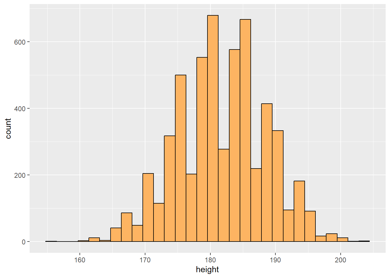
$ height         <int> 192, 181, 193, 187, 191, 183, 194, 185, 189, 173, 186, …
$ weight         <int> 84, 80, 84, 86, 80, 83, 88, 75, 80, 67, 78, 65, 88, 67,…
$ age            <int> 22, 31, 29, 33, 23, 31, 25, 20, 30, 22, 23, 31, 21, 29,…
$ club           <chr> "Atl. Nacional ", "Corinthians ", "Holstein Kiel ", "SK…
$ ball_control   <int> 55, 69, 25, 46, 14, 20, 52, 41, 68, 65, 62, 61, 45, 54,…
$ dribbling      <int> 43, 70, 12, 48, 8, 16, 43, 33, 67, 67, 59, 59, 28, 51, …
$ marking        <chr> "", "", "", "", "", "", "", "", "", "", "", "", "", "",…
$ slide_tackle   <int> 68, 56, 13, 66, 14, 13, 71, 65, 16, 30, 30, 58, 54, 50,…
$ stand_tackle   <int> 73, 58, 16, 69, 16, 17, 72, 70, 22, 33, 24, 59, 58, 51,…
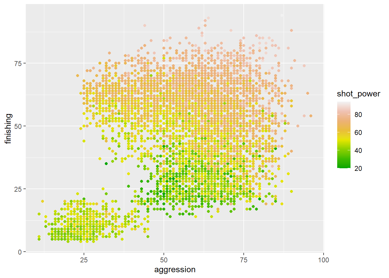
$ aggression     <int> 72, 62, 27, 71, 28, 27, 63, 46, 61, 40, 51, 60, 50, 86,…
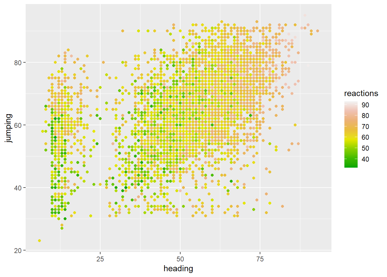
$ reactions      <int> 68, 70, 65, 64, 50, 70, 61, 54, 64, 47, 58, 58, 50, 55,…
$ att_position   <int> 30, 69, 17, 48, 10, 10, 37, 27, 72, 65, 62, 60, 25, 56,…
$ interceptions  <int> 65, 70, 20, 66, 12, 21, 68, 56, 22, 29, 31, 60, 54, 51,…
$ vision         <int> 30, 64, 49, 29, 38, 55, 34, 25, 50, 58, 57, 63, 48, 52,…
$ composure      <int> 50, 54, 48, 70, 34, 44, 56, 46, 64, 59, 53, 49, 48, 45,…
$ crossing       <int> 33, 60, 14, 44, 11, 10, 43, 26, 33, 60, 58, 51, 35, 51,…
$ short_pass     <int> 64, 63, 35, 58, 23, 25, 60, 49, 57, 63, 64, 65, 54, 50,…
$ long_pass      <int> 49, 63, 18, 53, 20, 23, 55, 45, 42, 61, 51, 63, 50, 42,…
$ acceleration   <int> 41, 64, 46, 35, 38, 55, 55, 63, 53, 81, 71, 74, 61, 73,…
$ stamina        <int> 55, 87, 38, 73, 28, 44, 75, 64, 54, 55, 63, 67, 46, 70,…
$ strength       <int> 86, 81, 68, 82, 64, 75, 84, 78, 86, 63, 71, 49, 78, 64,…
$ balance        <int> 40, 42, 41, 56, 24, 65, 33, 63, 58, 80, 54, 90, 52, 80,…
$ sprint_speed   <int> 52, 67, 48, 63, 31, 54, 68, 55, 69, 69, 74, 66, 64, 78,…
$ agility        <int> 43, 65, 36, 57, 34, 62, 34, 45, 60, 68, 67, 85, 51, 77,…
$ jumping        <int> 51, 65, 60, 80, 27, 72, 74, 71, 73, 60, 74, 71, 60, 58,…
$ heading        <int> 64, 54, 17, 67, 13, 21, 74, 55, 76, 47, 60, 48, 52, 51,…
$ shot_power     <int> 54, 60, 51, 32, 48, 48, 41, 39, 74, 73, 62, 56, 50, 51,…
$ finishing      <int> 30, 64, 14, 24, 4, 14, 33, 21, 71, 53, 60, 48, 25, 33, …
$ long_shots     <int> 31, 68, 20, 33, 6, 16, 18, 24, 58, 55, 59, 57, 23, 45, …
$ curve          <int> 32, 65, 20, 25, 9, 15, 29, 26, 53, 53, 49, 45, 37, 50, …
$ fk_acc         <int> 34, 62, 15, 13, 10, 13, 22, 26, 39, 31, 35, 50, 30, 40,…
$ penalties      <int> 41, 48, 26, 22, 16, 13, 34, 39, 72, 58, 57, 49, 41, 50,…
$ volleys        <int> 33, 46, 16, 19, 5, 10, 34, 25, 63, 60, 52, 39, 35, 46, …
$ gk_positioning <int> 10, 12, 64, 10, 61, 72, 10, 7, 11, 8, 8, 6, 9, 14, 12, …
$ gk_diving      <int> 11, 15, 74, 10, 59, 78, 5, 6, 7, 12, 10, 14, 10, 9, 8, …
$ gk_handling    <int> 6, 14, 65, 8, 62, 73, 14, 12, 10, 8, 6, 10, 13, 8, 9, 1…
$ gk_kicking     <int> 7, 8, 68, 14, 64, 64, 12, 13, 15, 5, 10, 10, 7, 15, 8, …
$ gk_reflexes    <int> 9, 14, 74, 9, 64, 74, 5, 11, 12, 15, 10, 11, 13, 11, 12…
$ value          <chr> "$1.400.000", "$975.00 ", "$1.100.000", "$650.00 ", "$3…

Atributos de los jugadores:

• Player: The name of the football player.
• Country: The nationality or home country of the player.
• Height: The height of the player in centimeters.
• Weight: The weight of the player in kilograms.
• Age: The age of the player.
• Club: The club to which the player is currently affiliated.
• Ball Control: Player’s skill in controlling the ball.
• Dribbling: Player’s dribbling ability.
• Marking: Player’s marking skill.
• Slide Tackle: Player’s ability to perform slide tackles.
• Stand Tackle: Player’s ability to perform standing tackles.
• Aggression: Player’s aggression level.
• Reactions: Player’s reaction time.
• Attacking Position: Player’s positioning for attacking plays.
• Interceptions: Player’s skill in intercepting passes.
• Vision: Player’s vision on the field.
• Composure: Player’s composure under pressure.
• Crossing: Player’s ability to deliver crosses.
• Short Pass: Player’s short passing accuracy.
• Long Pass: Player’s ability in long passing.
• Acceleration: Player’s acceleration on the field.
• Stamina: Player’s stamina level.
• Strength: Player’s physical strength.
• Balance: Player’s balance while playing.
• Sprint Speed: Player’s speed in sprints.
• Agility: Player’s agility in maneuvering.
• Jumping: Player’s jumping ability.
• Heading: Player’s heading skills.
• Shot Power: Player’s power in shooting.
• Finishing: Player’s finishing skills.
• Long Shots: Player’s ability to make long-range shots.
• Curve: Player’s ability to curve the ball.
• Free Kick Accuracy: Player’s accuracy in free-kick situations.
• Penalties: Player’s penalty-taking skills.
• Volleys: Player’s volleying skills.
• Goalkeeper Positioning: Goalkeeper’s positioning attribute (specific to goalkeepers).
• Goalkeeper Diving: Goalkeeper’s diving ability (specific to goalkeepers).
• Goalkeeper Handling: Goalkeeper’s ball-handling skill (specific to goalkeepers).
• Goalkeeper Kicking: Goalkeeper’s kicking ability (specific to goalkeepers).
• Goalkeeper Reflexes: Goalkeeper’s reflexes (specific to goalkeepers).
• Value: The estimated value of the player.

Modificamos la variable valuepara que tenga el tipo de dato que le corresponde y agregamos un cero a los valores que terminan .00.

df <- df %>%
  mutate(
    new_value = value %>%
      str_replace("\\.00\\s$", "000") %>%
      str_replace_all("\\$", "") %>%
      str_replace_all("\\.", "") %>%
      str_trim() %>%
      as.integer()
  )

df %>%
  head() %>%
  kable(format = "html") %>%
  kable_styling(full_width = FALSE) 

player	country	height	weight	age	club	ball_control	dribbling	marking	slide_tackle	stand_tackle	aggression	reactions	att_position	interceptions	vision	composure	crossing	short_pass	long_pass	acceleration	stamina	strength	balance	sprint_speed	agility	jumping	heading	shot_power	finishing	long_shots	curve	fk_acc	penalties	volleys	gk_positioning	gk_diving	gk_handling	gk_kicking	gk_reflexes	value	new_value
Cristian Castro Devenish	Colombia	192	84	22	Atl. Nacional	55	43		68	73	72	68	30	65	30	50	33	64	49	41	55	86	40	52	43	51	64	54	30	31	32	34	41	33	10	11	6	7	9	$1.400.000	1400000
Silaldo Taffarel	Brazil	181	80	31	Corinthians	69	70		56	58	62	70	69	70	64	54	60	63	63	64	87	81	42	67	65	65	54	60	64	68	65	62	48	46	12	15	14	8	14	$975.00	975000
Thomas Dähne	Germany	193	84	29	Holstein Kiel	25	12		13	16	27	65	17	20	49	48	14	35	18	46	38	68	41	48	36	60	17	51	14	20	20	15	26	16	64	74	65	68	74	$1.100.000	1100000
Michael Sollbauer	Austria	187	86	33	SK Rapid Wien	46	48		66	69	71	64	48	66	29	70	44	58	53	35	73	82	56	63	57	80	67	32	24	33	25	13	22	19	10	10	8	14	9	$650.00	650000
Diego Segovia	Uruguay	191	80	23	Independiente	14	8		14	16	28	50	10	12	38	34	11	23	20	38	28	64	24	31	34	27	13	48	4	6	9	10	16	5	61	59	62	64	64	$300.00	300000
Cláudio Ramos	Portugal	183	83	31	FC Porto	20	16		13	17	27	70	10	21	55	44	10	25	23	55	44	75	65	54	62	72	21	48	14	16	15	13	13	10	72	78	73	64	74	$2.800.000	2800000

Análisis exploratorio

A continuación se realizan algunos gráficos de análisis exploratorio con el fin de analizar la relación entre algunas variables y el comportamiento del precio de los jugadores.

ggplot(df, aes(y = new_value)) +
  geom_boxplot()

#paises con mas jugadores
top_10 <- df %>%
  count(country, sort = TRUE) %>% 
  head(n=10)


#barplot
ggplot(top_10, aes(x = reorder(country, n), y = n)) +
  geom_bar(stat = "identity", fill = "#FDB462") + 
  coord_flip() +
  labs(
    x = "País",
    y = "Cantidad de jugadores",
    title = "Top 10 países con mas jugadores"
  ) +
  theme_minimal()

ggplot(df, aes(height)) +
     geom_histogram(fill="#FDB462", colour="black")

    ggplot(data = df, aes(x = aggression, y = finishing, color = shot_power)) +
      geom_point()+ scale_color_gradientn(colours = terrain.colors(8))

    ggplot(data = df, aes(x = heading, y = jumping, color = reactions)) +
      geom_point()+ scale_color_gradientn(colours = terrain.colors(8))

    ggplot(data = df, aes(x = gk_handling, y = gk_diving, color = gk_kicking)) +
      geom_point()+ scale_color_gradientn(colours = terrain.colors(8))

top_5 <- df %>%
  count(country, sort = TRUE) %>% 
  head(n=5)

df_top_5_full <-df %>%
  filter(country %in% top_5$country)

df_top_5_full %>% 
  select(new_value, age, country, aggression, long_pass, shot_power, height, finishing, country) %>% 
  ggpairs(aes(color = country), upper = list(continuous = wrap("cor", size = 3, hjust=0.5)), progress=FALSE) + 
  theme(axis.text.x = element_text(angle = 90, hjust = 1), legend.position = "bottom") + 
  theme_bw()

df %>% 
  select_if(is.numeric) %>% # selección variables numéricas
  ggcorr(., layout.exp = 5, hjust = 1, size = 3.5, nbreaks = 5, color = "grey50") + # graficamos correlacion pearson
  labs(title='Correlograma de variables cuantitativas')

Preparación de la base de datos

Vamos a separar a los arqueros del resto de los jugadores.

df_ <-df %>% filter(gk_positioning < 30 & gk_positioning < 30) %>% #saco arqueros
  select(-c(value, marking, country, club, player)) %>% #saco ciertas columnas
  select(-starts_with("gk_"))#elimino columnas que caracterizan a los arqueros

Partición en train y test

df_split <- initial_split(df_,
                          prop = 0.8)

train<- df_split %>%
              training()

test <- df_split %>%
              testing()

train_sc <- as.data.frame(scale(train))
test_sc <- as.data.frame(scale(test))

train_sc %>% 
  ggcorr(., layout.exp = 5, hjust = 1, size = 3.5, nbreaks = 5, color = "grey50") + # graficamos correlacion pearson
  labs(title='Correlograma de variables cuantitativas en train')

Regresión Lineal Múltiple

# Modelo lineal
modelo_lineal = train_sc %>% lm(formula = new_value ~ .)

#Coeficientes
lineal_coef = modelo_lineal %>% tidy(conf.int=TRUE)

#graficamos los coeficientes estimados
lineal_coef %>% filter(!is.na(estimate)) %>% 
  ggplot(., aes(term, estimate))+
  geom_point(color = "forestgreen")+
  geom_pointrange(aes(ymin = conf.low, ymax = conf.high), color = "forestgreen")+
  geom_hline(yintercept = 0, lty = 4, color = "black") +
  labs(title = "Coeficientes de la regresión lineal", x="", y="Estimación e Int. Confianza") +
  theme_bw() +
  theme(axis.text.x = element_text(angle=90))

Graficamos los p-valores de mayor a menor para evaluar la significatividad individual de los coeficientes estimados.

lineal_coef %>% filter(!is.na(estimate)) %>% 
  ggplot(., aes(reorder(term, -p.value), p.value, fill=p.value))+
  geom_bar(stat = 'identity', aes(fill=p.value))+
  geom_hline(yintercept = 0.05) +
  labs(title = "P-valor de los regresores", x="", y="P-valor") +
  theme_bw() +
  theme(axis.text.x = element_text(angle=90)) + 
  scale_fill_gradient2(high='firebrick', low = 'forestgreen', mid='yellow2',midpoint = 0.5 )

Evaluamos la multicolinealidad de las regresoras.

car::vif (modelo_lineal)

       height        weight           age  ball_control     dribbling 
     3.706737      2.859991      1.730275      7.955621      7.222670 
 slide_tackle  stand_tackle    aggression     reactions  att_position 
    19.164518     20.855528      2.564884      3.661640      6.130713 
interceptions        vision     composure      crossing    short_pass 
    10.776083      5.478018      3.958109      3.902192      8.095459 
    long_pass  acceleration       stamina      strength       balance 
     5.757645      6.285201      1.833637      3.924871      3.642285 
 sprint_speed       agility       jumping       heading    shot_power 
     4.366600      4.508666      1.673276      3.131547      4.690486 
    finishing    long_shots         curve        fk_acc     penalties 
     8.778075      7.571247      5.211349      4.219688      3.497804 
      volleys 
     5.045861 

Regularización

La libreria glmnet nos permite trabajar con modelos Ridge, Lasso y Elastic Net. La función que vamos a utilizar es glmnet(). Es necesario que le pasemos un objeto matriz con los regresores y un vector con la variable a explicar (en este caso los salarios de los jugadores). Pueden chequear en el este link mas información sobre glmnet.

Fórmula:

\(ECM + \lambda{\left[\alpha\sum_{j}|\beta_j| +(1-\alpha)\sum_{j}\beta_j^2\right]}\)

• \(\lambda\) regula la importancia de la penalización.

• \(\alpha\) controla la importancia relativa de la regularización L1 y L2 y sirve para indicar si deseamos realizar un modelo de tipo Lasso, Ridge o Elastic Net.

  • Ridge: \(\alpha=0\)

  • Lasso: \(\alpha=1\)

  • Elastic Net: \(0<\alpha<1\)

Ridge (L2 regularization)

En este caso la penalización funciona añadiendo un término basado en la suma de los cuadrados de los coeficientes (\(\sum \beta_j^2\)) a la función de costo, lo que lleva la magnitud de los coeficientes hacia cero. Cuando \(\lambda\) toma valores altos, aplica una penalización fuerte, resultando en coeficientes muy pequeños y siendo muy útil para mitigar la multicolinealidad al distribuir la importancia entre variables correlacionadas.

\[\min_{\beta_0, \beta} \left\{ \frac{1}{2N} \sum_{i=1}^{N} (y_i - \beta_0 - x_i^T \beta)^2 + \lambda \sum_{j=1}^{p} \beta_j^2 \right\}\]

# modelo ridge 
ridge_model <- glmnet(
  as.matrix(train[, !names(train) %in% "new_value"]),  # predictoras
  train$new_value,  # variable respuesta
  standardize = T, #estandariza las variables
  alpha = 0  # Ridge
)

ridge_tidy <- ridge_model%>% tidy() %>% arrange(step)
ridge_tidy

# A tibble: 3,200 × 5
   term          step estimate      lambda dev.ratio
   <chr>        <dbl>    <dbl>       <dbl>     <dbl>
 1 (Intercept)      1 2.70e+ 6 4182932583.  4.62e-36
 2 height           1 8.96e-33 4182932583.  4.62e-36
 3 weight           1 3.55e-32 4182932583.  4.62e-36
 4 age              1 1.44e-31 4182932583.  4.62e-36
 5 ball_control     1 3.93e-31 4182932583.  4.62e-36
 6 dribbling        1 2.56e-31 4182932583.  4.62e-36
 7 slide_tackle     1 2.50e-32 4182932583.  4.62e-36
 8 stand_tackle     1 3.62e-32 4182932583.  4.62e-36
 9 aggression       1 1.24e-31 4182932583.  4.62e-36
10 reactions        1 4.96e-31 4182932583.  4.62e-36
# ℹ 3,190 more rows

add_top_coef_labels_glmnet <- function(fit, s = NULL, top_n = 5,
                                       offset_x = 0.5, cex = 0.8, col = "black",
                                       pos = 4) {
  # fit: objeto glmnet
  # s: valor lambda (si NULL usa el último de fit$lambda)
  # top_n: cuántas variables etiquetar (por valor absoluto)
  # offset_x: desplazamiento horizontal en la escala de -log(lambda)
  # cex, col, pos: parámetros de text()
  
  # elegir s (último lambda por defecto)
  if (is.null(s)) s <- fit$lambda[length(fit$lambda)]
  
  # extraer coeficientes (sin intercepto)
  coefs <- as.matrix(coef(fit, s = s))
  if (nrow(coefs) <= 1) return(invisible(NULL))  # por si no hay predictores
  coefs <- coefs[-1, , drop = FALSE]
  
  # seleccionar top_n por valor absoluto
  vals <- abs(coefs[, 1])
  ord <- order(vals, decreasing = TRUE)
  top_idx <- ord[seq_len(min(top_n, length(ord)))]
  top_coefs <- coefs[top_idx, 1, drop = FALSE]
  labels <- rownames(top_coefs)
  y <- as.numeric(top_coefs)
  
  # coordenada X en la escala del plot.glmnet (eje = -log(lambda))
  x_desired <- -log(s) + offset_x
  
  # asegurar que el plot ya existe y obtener límites
  usr <- par("usr")  # c(xmin, xmax, ymin, ymax)
  if (is.null(usr) || length(usr) < 4) {
    stop("No hay un plot activo. Llamá primero a plot(fit, xvar='lambda') antes de esta función.")
  }
  
  # si x_desired queda fuera del plot, recolocamos en el borde derecho menos margen
  x_min <- usr[1]; x_max <- usr[2]
  if (x_desired > x_max) x <- x_max - 0.02 * (x_max - x_min) else if (x_desired < x_min) x <- x_min + 0.02 * (x_max - x_min) else x <- x_desired
  
  # si hay muchos labels que se pisan, usar offsets verticales pequeños
  # calculamos desplazamientos verticales para evitar solapamiento simple
  # (ordenamos por y y separamos ligeramente)
  order_y <- order(y)
  y_sorted <- y[order_y]
  # simple jitter vertical proporcional al rango
  yrng <- usr[4] - usr[3]
  jitter_step <- 0.02 * yrng
  y_jittered <- y_sorted + seq(-floor(length(y_sorted)/2), floor((length(y_sorted)-1)/2)) * jitter_step
  # reordenar al orden original de top_idx
  y_final <- numeric(length(y))
  y_final[order_y] <- y_jittered
  
  # dibujar texto
  text(rep(x, length(y_final)), y_final, labels = labels, cex = cex, col = col, pos = pos)
  invisible(data.frame(label = labels, x = x, y = y_final))
}

A continuación se muestra el gráfico de valores de \(\lambda\) vs nivel de penalización.

• En el extremo izquierdo del gráfico se representan los valores altos de \(\lambda\), donde la penalización es máxima y por ende los coeficientes del modelo son prácticamente cero.

• En el extremo derecho se hayan los valores mas bajos de \(\lambda\). En esta zona, la penalización es mínima. El modelo se acerca a una regresión como la presentada anteriormente, y los coeficientes alcanzan sus máximos valores (no hay prácticamente penalización).

En una regresión Ridge, los coeficientes no llegan a ser cero, se acercan a cero (o se encojen) cuando \(\lambda\) es alto. En el gráfico se muestran las 5 variables mas importantes. Ridge no realiza una selección de variables.

reactions y age son las variables más importantes y con mayor impacto en el salario de los jugadores FIFA 2024.

plot(ridge_model, 
     xvar = "lambda", 
     label=F,
     xlim = c(-22, -11),
     ylim= c(-2.5e05, 3.5e05))
# Agregás etiquetas de las 5 variables más importantes

add_top_coef_labels_glmnet(ridge_model, top_n = 5, offset_x = 0.2, col = "black")

Búsqueda del lambda óptimo

A partir de realizar validación cruzada se encuentra el lambda que minimiza el ECM.

# CV para encontrar el mejor lambda
cv_ridge <- cv.glmnet(
  as.matrix(train[, !names(train) %in% "new_value"]),
  train$new_value,
  standarize=T,
  nfolds= 10,
  type.measure = "mse",
  alpha = 0  # ridge
)

cv_ridge$lambda.min  # este valor de lambda minimiza el ecm

[1] 418293.3

ECM vs complejidad del modelo

A medida que nos movemos de izquierda a derecha (disminuye \(\lambda\)), el error desciende progresivamente (el modelo se ajusta mejor) hasta que alcanza una meseta.

Como se puede apreciar, aparecen dos lineas verticales en el gráfico. La línea punteada de la derecha corresponde al \(\lambda_{min}\), es decir el valor de \(\lambda\) que da el ECM promedio en la validación cruzada. La línea punteada de la izquierda corresponde al \(\lambda_{1se}\), en el cual se selecciona el modelo más simple (más penalizado, con coeficientes más pequeños) que se considera estadísticamente indistinguible del modelo con el error mínimo.

plot(cv_ridge)

Modelo final

# Selección lambda óptimo
ridge_lambda_opt = cv_ridge$lambda.min

# Entrenamiento modelo óptimo
ridge_opt = glmnet(as.matrix(train[, !names(train) %in% "new_value"]),  # Predictor variables
                  train$new_value,
                   alpha = 0, # Indicador del tipo de regularizacion
                   standardize = TRUE,  # Estandarizamos
                   lambda = ridge_lambda_opt)
# Salida estandar
ridge_opt

Call:  glmnet(x = as.matrix(train[, !names(train) %in% "new_value"]),      y = train$new_value, alpha = 0, lambda = ridge_lambda_opt,      standardize = TRUE) 

  Df  %Dev Lambda
1 31 30.26 418300

El porcentaje de deviance explicado del modelo final es del 31,4%.

# Tidy
ridge_opt %>% tidy() %>% mutate(estimate = round(estimate, 4))

# A tibble: 32 × 5
   term          step   estimate  lambda dev.ratio
   <chr>        <dbl>      <dbl>   <dbl>     <dbl>
 1 (Intercept)      1 -41837208. 418293.     0.303
 2 height           1     51311. 418293.     0.303
 3 weight           1     -1728. 418293.     0.303
 4 age              1   -222401. 418293.     0.303
 5 ball_control     1     51273. 418293.     0.303
 6 dribbling        1    -16994. 418293.     0.303
 7 slide_tackle     1      1011. 418293.     0.303
 8 stand_tackle     1     19708. 418293.     0.303
 9 aggression       1     18411. 418293.     0.303
10 reactions        1    316049. 418293.     0.303
# ℹ 22 more rows

Lasso (L1 regularization)

La penalización en una regresión Lasso funciona añadiendo un término basado en la suma de los valores absolutos de los coeficientes (\(\sum |\beta_j|\)) a la función de costo, lo que reduce la magnitud de los coeficientes y puede forzar a los menos relevantes a ser exactamente cero, realizando selección de variables.

\[\min_{\beta_0, \beta} \left\{ \frac{1}{2N} \sum_{i=1}^{N} (y_i - \beta_0 - x_i^T \beta)^2 + \lambda \sum_{j=1}^{p} |\beta_j| \right\}\]

lasso_model <- glmnet(
  as.matrix(train[, !names(train) %in% "new_value"]),  # Predictor variables
  train$new_value,  # Response variable
  standardize = T,
  alpha = 1  # lasso
)

plot(lasso_model, 
     xvar = "lambda", 
     label=F,
     xlim = c(-15, -6),
     ylim= c(-3e05, 4e05))
# se agrega etiquetas de las 5 variables más importantes

add_top_coef_labels_glmnet(lasso_model, top_n = 5, offset_x = 0.2, col = "black")

cv_lasso <- cv.glmnet(
  as.matrix(train[, !names(train) %in% "new_value"]),
  train$new_value,
  standarize=T,
  nfolds = 10
)

cv_lasso$lambda.min  # valor de lambda que minimiza el ecm

[1] 9011.855

plot(cv_lasso)

# Selección lambda óptimo
lasso_lambda_opt = cv_lasso$lambda.min
# Entrenamiento modelo óptimo
lasso_opt = glmnet(x = as.matrix(train[, !names(train) %in% "new_value"]), # Matriz de regresores
                   y = train$new_value, #Vector de la variable a predecir
                   alpha = 1, # Indicador del tipo de regularizacion
                   standardize = TRUE,  # Estandarizamos
                   lambda = lasso_lambda_opt)
# Salida estandar
lasso_opt

Call:  glmnet(x = as.matrix(train[, !names(train) %in% "new_value"]),      y = train$new_value, alpha = 1, lambda = lasso_lambda_opt,      standardize = TRUE) 

  Df  %Dev Lambda
1 28 30.38   9012

El porcentaje de deviance explicado del modelo final es del 30.35%. La regresión Lasso selecciona 27 variables.

# Tidy
lasso_opt %>% tidy() %>% mutate(estimate = round(estimate, 2))

# A tibble: 29 × 5
   term           step   estimate lambda dev.ratio
   <chr>         <dbl>      <dbl>  <dbl>     <dbl>
 1 (Intercept)       1 -41418495.  9012.     0.304
 2 height            1     48411.  9012.     0.304
 3 age               1   -236862.  9012.     0.304
 4 ball_control      1     51885.  9012.     0.304
 5 dribbling         1    -21756.  9012.     0.304
 6 stand_tackle      1     29159.  9012.     0.304
 7 aggression        1     18587.  9012.     0.304
 8 reactions         1    366597.  9012.     0.304
 9 att_position      1    -28638.  9012.     0.304
10 interceptions     1    -31333.  9012.     0.304
# ℹ 19 more rows

Elastic net

La penalización Elastic Net combina las fortalezas de Ridge y Lasso al añadir a la función de costo una mezcla lineal de las penalizaciones \(L_1\) y \(L_2\), controlada por el parámetro \(\alpha\). Un \(\lambda\) (lambda) alto resulta en un modelo más penalizado.

\[ \min_{\beta_0, \beta} \left\{ \frac{1}{2N} \sum_{i=1}^{N} (y_i - \beta_0 - x_i^T \beta)^2 + \lambda \left[ (1 - \alpha)\frac{1}{2} \sum_{j=1}^{p} \beta_j^2 + \alpha \sum_{j=1}^{p} |\beta_j| \right] \right\} \]

models <- list()
for (i in 0:20) {
  name <- paste0("alpha", i/20)
  

  models[[name]] <-
    cv.glmnet(x = as.matrix(train[, !names(train) %in% "new_value"]), # Matriz de regresores
                   y = train$new_value, standarize=T, alpha=i/20)
}

# Lista para guardar los modelos
models <- list()

# Vector para almacenar los resultados
results <- data.frame(alpha = numeric(), lambda = numeric())

for (i in 0:20) {
  a <- i / 20
  name <- paste0("alpha", a)
  
  # Ajuste del modelo con cv.glmnet
  models[[name]] <- cv.glmnet(
    x = as.matrix(train[, !names(train) %in% "new_value"]),
    y = train$new_value,
    standardize = TRUE,
    nfolds= 10,
    alpha = a
  )
  
  # Guardar el alpha y el MSE mínimo
  results <- rbind(
    results,
    data.frame(
      alpha = a,
      lambda = models[[name]]$lambda.min  # cvm contiene el MSE promedio por lambda
    )
  )
}

# Ver el data frame final
results

   alpha    lambda
1   0.00 418293.26
2   0.05 197810.00
3   0.10 108548.11
4   0.15  79420.95
5   0.20  65373.29
6   0.25  62993.89
7   0.30  47831.41
8   0.35  37356.17
9   0.40  35873.55
10  0.45  21978.89
11  0.50  28698.84
12  0.55  26089.86
13  0.60  23915.70
14  0.65  20114.86
15  0.70  15506.87
16  0.75  13187.33
17  0.80  17936.78
18  0.85  15381.95
19  0.90  12060.90
20  0.95  12540.15
21  1.00   9890.50

Mejor modelo

elastic_opt = glmnet(x = as.matrix(train[, !names(train) %in% "new_value"]), # Matriz de regresores
                   y = train$new_value, #Vector de la variable a predecir
                   alpha = 0.95, 
                   standardize = TRUE,
                   lambda=min(results$lambda))
# Salida estandar
elastic_opt

Call:  glmnet(x = as.matrix(train[, !names(train) %in% "new_value"]),      y = train$new_value, alpha = 0.95, lambda = min(results$lambda),      standardize = TRUE) 

  Df  %Dev Lambda
1 28 30.37   9890

# Tidy
elastic_opt %>% tidy() %>% mutate(estimate = round(estimate, 2))

# A tibble: 29 × 5
   term           step   estimate lambda dev.ratio
   <chr>         <dbl>      <dbl>  <dbl>     <dbl>
 1 (Intercept)       1 -41379168.  9890.     0.304
 2 height            1     48285.  9890.     0.304
 3 age               1   -236748.  9890.     0.304
 4 ball_control      1     51623.  9890.     0.304
 5 dribbling         1    -21376.  9890.     0.304
 6 stand_tackle      1     28782.  9890.     0.304
 7 aggression        1     18505.  9890.     0.304
 8 reactions         1    366459.  9890.     0.304
 9 att_position      1    -28385.  9890.     0.304
10 interceptions     1    -30909   9890.     0.304
# ℹ 19 more rows

Resumen

# 1. Extraer los coeficientes del modelo Elastic Net óptimo
# La función 'coef' devuelve una matriz 'dgCMatrix'
elastic_coef <- coef(elastic_opt)

# 2. Extraer los coeficientes de los modelos Ridge y Lasso óptimos
# Asume que ya tienes 'ridge_opt' y 'lasso_opt' ajustados de manera similar
ridge_coef <- coef(ridge_opt)
lasso_coef <- coef(lasso_opt)

# Convertir y limpiar los coeficientes a un data.frame simple
extract_and_clean <- function(model_coef, model_name) {
  df <- data.frame(
    Variable = rownames(model_coef),
    Coeficiente = as.numeric(model_coef),
    Modelo = model_name
  )
  # Quitar la columna del intercepto (Intercept) para simplificar la comparación si se desea
  # df <- subset(df, Variable != "(Intercept)")
  return(df)
}

# Aplicar la función de limpieza y combinación
coef_ridge <- extract_and_clean(ridge_coef, "Ridge (α=0)")
coef_lasso <- extract_and_clean(lasso_coef, "Lasso (α=1)")
coef_elastic <- extract_and_clean(elastic_coef, "Elastic Net (α=0.95)")

# Combinar todas las tablas en una sola
tabla_final <- merge(coef_ridge[, c(1, 2)], coef_lasso[, c(1, 2)], by = "Variable", all = TRUE, suffixes = c(".Ridge", ".Lasso"))
tabla_final <- merge(tabla_final, coef_elastic[, c(1, 2)], by = "Variable", all = TRUE)
names(tabla_final)[4] <- "Coeficiente.ElasticNet"

# Opcional: reemplazar NAs (si hubiera) con 0 para Lasso (aunque con tu ajuste no debería haber NAs)
# tabla_final[is.na(tabla_final)] <- 0

tabla_final

        Variable Coeficiente.Ridge Coeficiente.Lasso Coeficiente.ElasticNet
1    (Intercept)     -4.183721e+07     -4.141850e+07          -4.137917e+07
2   acceleration      4.479216e+04      4.474708e+04           4.459641e+04
3            age     -2.224014e+05     -2.368623e+05          -2.367481e+05
4     aggression      1.841117e+04      1.858744e+04           1.850527e+04
5        agility     -2.502621e+04     -2.920451e+04          -2.896862e+04
6   att_position     -2.026471e+04     -2.863769e+04          -2.838535e+04
7        balance      1.803556e+04      1.778636e+04           1.760122e+04
8   ball_control      5.127288e+04      5.188543e+04           5.162325e+04
9      composure      5.975781e+04      5.178765e+04           5.182172e+04
10      crossing      1.532453e+04      1.637492e+04           1.623767e+04
11         curve      1.338590e+04      1.425067e+04           1.419897e+04
12     dribbling     -1.699359e+04     -2.175615e+04          -2.137613e+04
13     finishing      3.104593e+04      3.852337e+04           3.820697e+04
14        fk_acc      1.031238e+04      1.290456e+04           1.281652e+04
15       heading      3.676510e+04      3.126445e+04           3.127771e+04
16        height      5.131127e+04      4.841061e+04           4.828494e+04
17 interceptions     -2.020321e+04     -3.133341e+04          -3.090900e+04
18       jumping      1.532115e+03      5.868123e+02           5.319712e+02
19     long_pass     -3.988093e+02      0.000000e+00           0.000000e+00
20    long_shots     -2.364124e+04     -2.763035e+04          -2.746300e+04
21     penalties      1.565524e+04      1.246561e+04           1.247764e+04
22     reactions      3.160493e+05      3.665967e+05           3.664585e+05
23    short_pass      4.484603e+04      2.940028e+04           2.947046e+04
24    shot_power     -2.095961e+04     -2.429482e+04          -2.408652e+04
25  slide_tackle      1.011101e+03      0.000000e+00           0.000000e+00
26  sprint_speed      4.543311e+04      4.600434e+04           4.597140e+04
27       stamina      4.090059e+02     -9.534677e+02          -8.772476e+02
28  stand_tackle      1.970784e+04      2.915927e+04           2.878203e+04
29      strength      7.836599e+03      5.911185e+03           5.845007e+03
30        vision      2.253327e+04      2.567220e+04           2.545884e+04
31       volleys      2.360521e+04      2.607618e+04           2.601014e+04
32        weight     -1.727652e+03      0.000000e+00           0.000000e+00

Evaluando en Test

x_test <- as.matrix(test[, !names(test) %in% "new_value"])
y_test <- test$new_value

# === Ridge (alpha=0) ===
pred_ridge <- predict(ridge_opt, x_test)
mse_ridge <- mean((y_test - pred_ridge)^2)          # ECM
rmse_ridge <- sqrt(mse_ridge)                       # RSME
mae_ridge <- mean(abs(y_test - pred_ridge))         # MAE

# === Lasso (alpha=1) ===
pred_lasso <- predict(lasso_opt, x_test)
mse_lasso <- mean((y_test - pred_lasso)^2)
rmse_lasso <- sqrt(mse_lasso)
mae_lasso <- mean(abs(y_test - pred_lasso))

# === Elastic Net (alpha=0.95) ===
pred_elastic <- predict(elastic_opt, x_test)
mse_elastic <- mean((y_test - pred_elastic)^2)
rmse_elastic <- sqrt(mse_elastic)
mae_elastic <- mean(abs(y_test - pred_elastic))

# === Tabla resumen ===
results <- data.frame(
  Modelo = c("Ridge", "Lasso", "Elastic Net"),
  ECM_Test = c(mse_ridge, mse_lasso, mse_elastic),
  RSME_Test = c(rmse_ridge, rmse_lasso, rmse_elastic),
  MAE_Test = c(mae_ridge, mae_lasso, mae_elastic))

print(results)

       Modelo     ECM_Test RSME_Test MAE_Test
1       Ridge 2.141391e+13   4627517  2957468
2       Lasso 2.163449e+13   4651289  3001880
3 Elastic Net 2.163084e+13   4650897  3001220

plot(y_test, pred_lasso)
abline(0, 1)

Ridge y Lasso reducen la magnitud de los coeficientes de las variables, lo cual atenúa pero no resuelve el impacto de outliers. Ridge suaviza la influencia, Lasso puede volverse inestable y seleccionar mal variables. La regularización controla varianza, no robustez; para outliers se necesitan técnicas robustas adicionales.